Midwest Mayors complain that “city” crime rankings are not accurate because cities are defined by city limits, which are determined by politics, not consistent rules of population statistics. Rust belt cities typically have city limits locked in place encircling a small old inner portion of the metropolitan area and containing few if any low-crime suburbs. Newer Western cities, by contrast, cast their city limits far out into farm fields where they encircle the majority of their metro low crime suburbs, which dilutes their average crime rates.

https://goo.gl/maps/XVnTkkaaGv72
But researchers put both types of cities into the same “city” ranking, and then declare the cities with most crime per resident as the most dangerous. Since the general public associate cities with entire regions, “city limit” rankings can unfairly paint an entire region as crime riddled while masking growing crime issues in so-called “hot” younger cities. These rankings tell you almost nothing about personal danger, since any city can change its ranking just by moving a boundary without actually lowering crime.
By contrast, crime rankings based on Metropolitan Statistical Area (MSA) boundaries, instead of city limits, make use of city definitions set consistently, metro to metro, by the Federal government using statistical rules based on population. For some reason, these more valid MSA rankings are ignored by the media. In 2012, Forbes Magazine switched from MSA crime ranking to a city limits crime ranking, with scant rationale, saying “We used cities instead of larger metropolitan statistical areas, which gave the disadvantage to older cities with tighter boundaries.”
MSAs usually have an inner business cores at their centers, older smaller homes and multi-family homes further out, and suburbs beyond that. I contend that statisticians could do a much better job of comparing major cities by going down to the zip code level and identifying zip codes in the inner 10%, 20%, 30% etc. of their MSAs for crime statistics. Then one could compare the inner 10% core of the Pittsburgh metro area with the inner 10% core of the Houston metro area if one was planning to live near downtown. Or compare the 50% population ring of two metros for folks comparing suburbs. But that takes some work, and most crime rankers just paste FBI tables into a spreadsheet, combine crime categories into a single score for each city, and then sort on that score. This is something almost anyone could do in an afternoon.
I decided to take my own advice and see how hard it would be to go onto the internet and address just two cities using the percent of population rings approach to compare crime rates. I chose to compare St. Louis and Kansas City. St. Louis is the last old Eastern City as you go West, and KC could be seen as the first Western style city. In the free 2014 CQ Press Cities Crime Ranking, St. Louis ranked at #5 worst for crime while Kansas City ranked better at #61. But in the 2014 CQ Press Metro Ranking, the orders were reversed with Kansas City ranking worse at #52, while St. Louis ranked safer at #95. So I was anxious to see how the plots would show a transition as the data extended further from City Hall.
Method
Here are the steps I used to plot St. Louis and Kansas City crime. The same steps and data sources (links at the end of the piece) work for all metro areas.
Method for Average Crime index for percent population rings from City Hall. 10%, 20%, etc.
- Find zip codes for each Metropolitan Statistical Area (MSA)
- Find LAT LONG of City Hall of the primary city of each MSA and each MSA Zip Code area
- Compute distance of each zip code from city hall in miles with LAN LONG to mile conversion.
- Get Crime Index for each zip code
- Get population for each zip code
- Determine distance rings containing 10% of the population, 20%, etc.
- Identify specific zip codes within each ring
- Compute total crime index for each % ring using zip code crime index weighted by population.
- Plot crime index for the 10% population ring, 20% ring, etc. as a histogram.
I was able to find free databases online for each of the steps in this approach, but it was a bit tedious copying crime indexes by zip code from one of various neighborhood data realty sites and pasting the indexes into my spreadsheet one at a time. Professional researchers could probably purchase the entire crime-by-zip-code database in XL format to make that part a lot easier.
I computed the distances from City Hall for 10% of the metro populations, 20%, 30%, etc. at these distances:
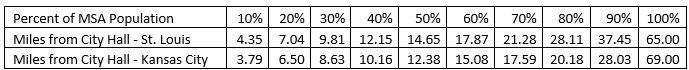 Table 1. Distance from City Hall where 10%, 20%, etc. of the metro population live.
I realized that since St. Louis and Kansas City metro areas are fairly similar, it would be interesting and pretty easy to go through step 4 above and just plot zip code crime indexes for each zip code as a function of distance from city hall. The data include zip code areas in Illinois for St. Louis, and Kansas for Kansas City as well as Missouri zip codes.
Results
Here is the scatter plot of zip code crime indexes vs. distance from City Hall for St. Louis and Kansas City. US average crime index is 100.

Figure 1. Zip Code Crime Index by miles from City Hall for St. Louis and Kansas City Metros.
The website posting the crime index for each zip code said the index is a combination of rape, murder, assault, robbery, burglary, larceny and vehicle theft normalized against a US average score of 100. So 200 means twice the average US crime. The counts of each crime category are unweighted according to the web site, so murder counts the same as robbery.
Continuing with the remaining steps to get a histogram of crime indexes by percent of metro area rings, I combine crime indexes within each percent ring. For this, I weighted the indexes by zip code population, so a zip code with just 3 people would contribute proportionally less than one with 1,000 people within a percent ring. I collected data up through the 60% ring. For the full metro numbers, I computed the St Louis and Kansas City crime indexes directly from the FBI data tables.
Here is the crime index histogram for each percent ring of population out to 60% from City Hall.
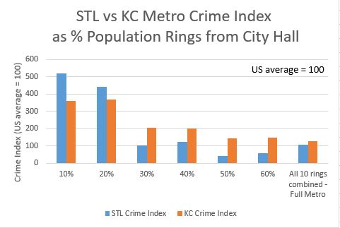
Figure 2. Crime Index by 10% rings of population out from City Hall.
And here is what the data looks at the 10% core, the entire inner 50% of the metro population and the full metro.
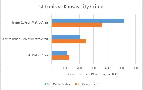
Figure 3. Crime Index for 10% core, the entire inner 50% of the metro population, and the full metro.
Since St. Louis and Kansas City are similar in size, the histogram information roughly lines up with the distance scatter plot. If I was comparing St. Louis to a much smaller or larger metro, the percentage histogram would be more useful.
Here are maps of St. Louis and Kansas City with the Crime Index shown as a number from 1 to 6, where 6 represents crime 6 times the national average. The links below the maps go to short videos of each map in a circling motion to see around the data pillars.

Figure 4. St. Louis Crime Index by Zip Code. US average is 1.
https://flic.kr/p/G9QBsb

Figure 5. Kansas City Crime Index by Zip Code. US average is 1.
https://flic.kr/p/FnxJMC
Observations
I was surprised at how different the plots turned out between the two cities. As expected, core areas of both metros have higher crime rates, and suburbs have lower crime rates. Since the full St. Louis metro crime rate is lower than the full Kansas City metro crime rate, I was guessing that the two metros were similar enough in configuration that St. Louis would come out slightly safer at every percent of population and distance out from City Hall. Instead I learned that the inner 20% of St. Louis zip codes had around a 20% higher crime index than their Kansas City counterparts. I was even more surprised to see how much safer St. Louis inner suburbs are than their Kansas City counterparts. The Kansas City crime index was around 40% higher than St. Louis for the 30% through 60% population rings. The higher suburban crime in Kansas City more than makes up for the higher inner core crime in St Louis to account for the overall higher crime rate in the entire Kansas City metro area.
The crimes per person may be higher in St. Louis inner core because the number of people living there (the denominator) has plummeted over the last 70 years until recently, while the number of people working, driving through, and doing business during the day is still pretty high. But crime indexes always divide only by the resident count, not the visitor count. I suspect these patterns may be typical for older rust belt cities where the middle class has moved to larger modern homes in the suburbs long ago, whereas Western cities still have many newer homes close to the central core. Some cities like St. Louis and Detroit have an additional factor pulling residents westward – a central business district built almost out on a peninsula up against a major barrier – the Mississippi River for St. Louis and the Canadian border for Detroit.
Conclusions
If all the City and Metro crime rankings were replaced with charts like these, planners could make better decisions about the status of crime in major cities. This approach completely eliminates the city limits as a factor driving a false ranking. Planners can better see how their metro area stacks up against other metros at similar distance rings when assigning resources to fight crime. The next step would be to go down to zip code level directly to address specific crime problems within the metro areas. If publishers must have crime rankings to sell magazines, the full MSA boundary ranking, or the 50% inward stats are more representative of relative crime rates.
References
Links to data sources:
Zip Codes that make up each MSA:
http://www.dol.gov/owcp/regs/feeschedule/fee/fee11/fs11_gpci_by_msa-ZIP.pdf
LAT LONG of each metro – City Hall
https://www.statcrunch.com/app/index.php?dataid=1232319
Zip Code Area LAT LONGS
https://boutell.com/zipcodes/
Convert difference between two LAT LONGs to statute miles
=ACOS(COS(RADIANS(90-A2)) *COS(RADIANS(90-A3)) +SIN(RADIANS(90-A2)) *SIN(RADIANS(90-A3)) *COS(RADIANS(B2-B3))) *3958.756
Crime rating and population size for each zip code
http://www.moving.com/real-estate/city-profile/
Population distance spread from City Hall
http://www.census.gov/population/metro/data/pop_pro.html
Zip code map images
http://www.zipmap.net/Missouri/St._Louis_city.htm
FBI Table 6 to get Full Metro Stats to compute full metro counts 2013
https://www.fbi.gov/about-us/cjis/ucr/crime-in-the-u.s/2013/crime-in-the-u.s.-2013/tables/6tabledatadecpdf/table-6
FBI Table 1 to get Full US Stats to scale computer full metro crime Indexes 2013
https://www.fbi.gov/about-us/cjis/ucr/crime-in-the-u.s/2013/crime-in-the-u.s.-2013/tables/1tabledatadecoverviewpdf/table_1_crime_in_the_united_states_by_volume_and_rate_per_100000_inhabitants_1994-2013.xls
Total Crime Risk Index Used by Moving.com description:
Total Crime Risk – A score that represents the combined risks of rape, murder, assault, robbery, burglary, larceny and vehicle theft compared to the national average of 100. A score of 200 indicates twice the national average total crime risk, while 50 indicates half the national risk. The different types of crime are given equal weight in this score, so murder, for example, does not count more than vehicle theft. Scores are based on demographic and geographic analyses of crime over seven years.
http://www.greenhavenga.org/s/Stereotype-Busting-Some-Bad-Neighborhoods-Have-Lower-Crime-than-Affluent-Neighborhoods.pdf
CQ Press 2014 (2013 data) rankings of safest cities and safest metro areas.
http://os.cqpress.com/citycrime/2013/2014_MetroCrimeRateRankings(LowtoHigh).pdf
http://os.cqpress.com/citycrime/2013/2014_CityCrimeRankings(LowtoHigh).pdf
Forbes Most Dangerous Cities
2011 When Forbes used the MSA Ranking
http://www.forbes.com/sites/johngiuffo/2011/10/03/americas-most-dangerous-cities/#5a2634a11878
2012 When Forbes switched to the City Limits Ranking
http://www.forbes.com/sites/danielfisher/2012/10/18/detroit-tops-the-2012-list-of-americas-most-dangerous-cities/#242169ce11d7
Gary Kreie is a recently retired missile software engineer/manager.